BIXI Montreal Bike-Share — Operations Analysis

A SQL + Python analysis of Montreal’s BIXI bike-share network over the full 2024 open dataset (13.2M trips). The goal wasn’t just to describe ridership — it was to turn a raw 2.6 GB CSV into operational recommendations a BIXI dispatch team could actually act on: when to staff, which stations to rebalance, and where to invest.

01 The problem

BIXI runs 1,100+ stations across Montreal. Bikes naturally pile up at some stations and run dry at others, forcing manual truck-based rebalancing. Three operational questions drove the analysis:

• When does demand peak, so staffing and rebalancing can be scheduled around it?
• Which stations are chronically overloaded and need bikes removed?
• Which routes and areas drive the most ridership, to prioritise investment?

02 How it was built

Data modeling

Raw CSV → staging table → a normalised schema: stations (1,134 unique, deduplicated by name) and trips (13.2M valid; ~73K rows with missing station data dropped, ~0.56%). Indexes on the station and time columns keep the aggregation-heavy queries fast. One real gotcha: timestamps needed an explicit AT TIME ZONE 'America/Montreal' conversion — the initial load stored them in the server’s default zone, which would have quietly skewed the entire hourly pattern.

Analysis techniques

The dispatch recommendation rests on one CTE query — arrivals minus departures per station. A positive net flow means bikes accumulate (remove them); negative means the station runs dry (add them):

WITH departures AS (
    SELECT start_station_id AS station_id, COUNT(*) AS total_departures
    FROM trips GROUP BY start_station_id
),
arrivals AS (
    SELECT end_station_id AS station_id, COUNT(*) AS total_arrivals
    FROM trips GROUP BY end_station_id
)
SELECT
    s.station_name,
    s.arrondissement,
    COALESCE(a.total_arrivals, 0)
      - COALESCE(d.total_departures, 0) AS net_flow
FROM stations s
LEFT JOIN departures d ON s.station_id = d.station_id
LEFT JOIN arrivals   a ON s.station_id = a.station_id
ORDER BY net_flow DESC;

03 What the data showed

A commuter pattern, not just leisure

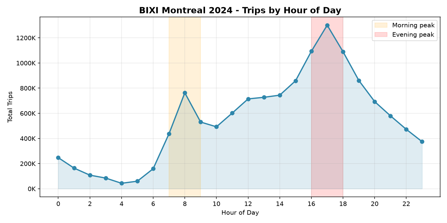
Ridership peaks sharply at 8am and 5pm on a 24-hour cycle — classic work-commute behaviour rather than purely recreational use. This is what makes pre-peak rebalancing windows worth staffing.

Extreme seasonality — and a shift in rider type

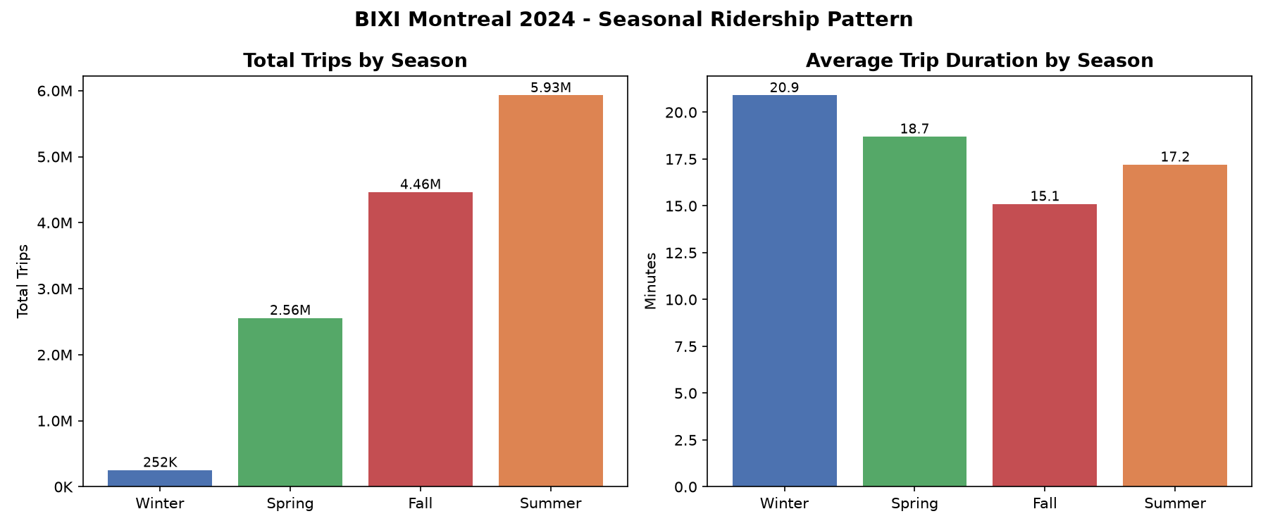
Summer ridership (5.93M trips) is ~23× winter (252K). Yet average trip duration is longer in winter (20.9 min vs. 17.2) — suggesting winter riders are a smaller, more committed group of true commuters, while summer volume includes many short casual trips.

Ridership concentrated around Mont-Royal / Plateau

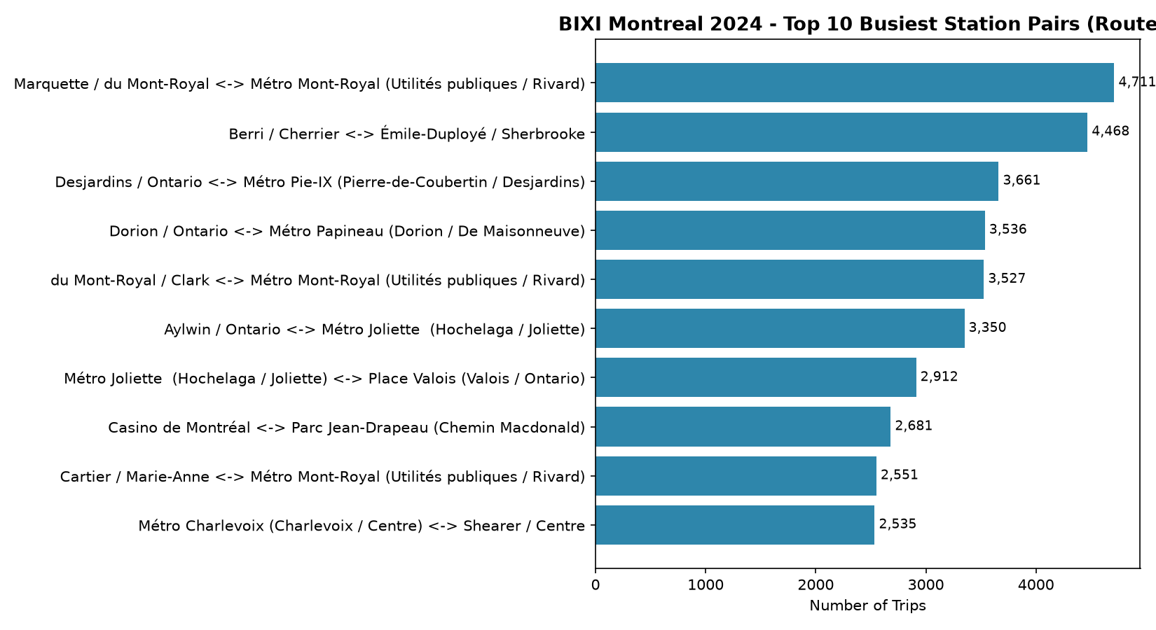
The busiest station-pair routes are almost all anchored around Mont-Royal metro and the Plateau — Montreal’s densest, most bike-friendly residential area.

Dispatch priority: Ville-Marie is chronically overloaded

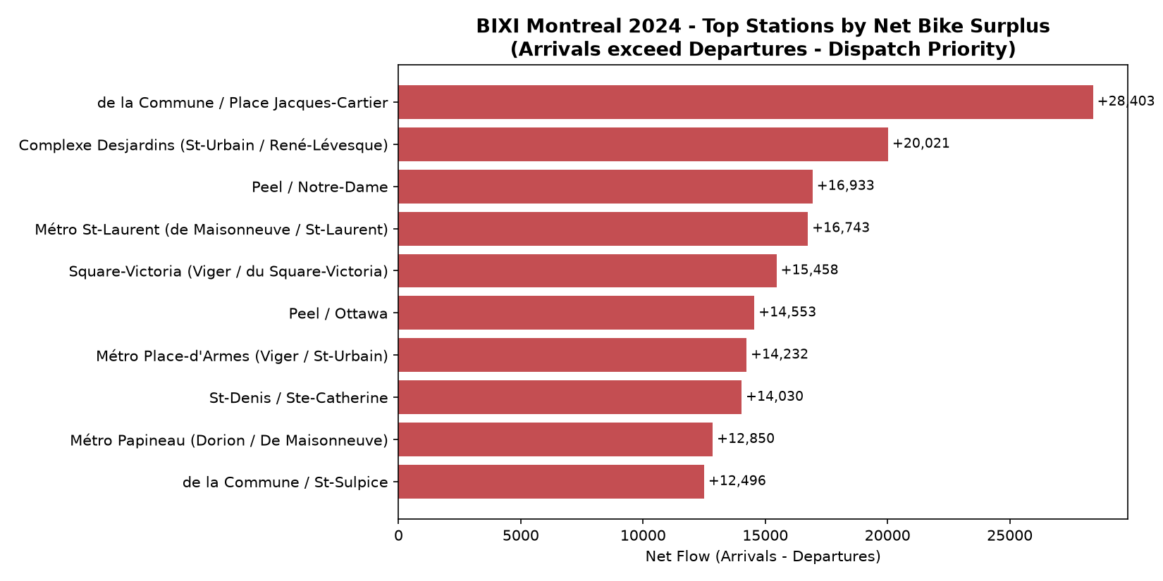
Stations in Ville-Marie (downtown / Old Port) show the largest positive net flow — bikes arrive far more than they leave. Trucks should proactively remove bikes here rather than wait for stations to fill.

04 Recommendations

• Staffing: concentrate rebalancing crews in the pre-peak windows (6–7am, 3–4pm) to get ahead of the 8am / 5pm surges.
• Dispatch routing: prioritise downtown Ville-Marie stations for bike removal — a standing daily route beats reactive dispatch.
• Seasonal operations: given the ~23× volume swing, winter fleet size could be cut substantially without hurting service, freeing bikes for maintenance.

05 Limitations

• No membership or bike-ID data in the 2024 export, so rider-level segmentation (member vs. casual) wasn’t possible.
• Findings reflect 2024 only; multi-year trend analysis would require reconciling BIXI’s different historical data formats.